arviz_plots.plot_dgof_dist#
- arviz_plots.plot_dgof_dist(dt, *, var_names=None, filter_vars=None, group='posterior', coords=None, sample_dims=None, kind=None, envelope_prob=None, plot_collection=None, backend=None, labeller=None, aes_by_visuals=None, visuals=None, stats=None, **pc_kwargs)[source]#
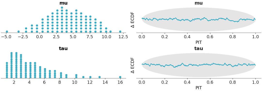
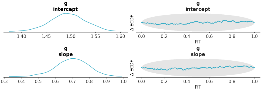
Plot 1D marginal distributions and a Δ-ECDF-PIT diagnostic.
The marginal distributions are plotted using the specified kind (kde, histogram, or quantile dot plot). Additionally, a Δ-ECDF-PIT diagnostic is plotted to assess the goodness-of-fit of the estimated distributions to the underlying data [1]. If the estimated distributions are accurate, the PIT values should be uniformly distributed on [0, 1], resulting in a Δ-ECDF close to zero. Simultaneous confidence bands are computed using simulation method described in [2].
- Parameters:
- dt
xarray.DataTree Input data
- var_names
strorlistofstr, optional One or more variables to be plotted. Prefix the variables by ~ when you want to exclude them from the plot.
- filter_vars{
None, “like”, “regex”}, optional, default=None If None (default), interpret var_names as the real variables names. If “like”, interpret var_names as substrings of the real variables names. If “regex”, interpret var_names as regular expressions on the real variables names.
- group
str, default “posterior” Group to be plotted.
- coords
dict, optional Coordinates to be used to index data variables.
- sample_dims
stror sequence of hashable, optional Dimensions to reduce unless mapped to an aesthetic. Defaults to
rcParams["data.sample_dims"]- kind{“kde”, “hist”, “dot”}, optional
How to represent the marginal density. Defaults to
rcParams["plot.density_kind"]- envelope_prob
float, optional Indicates the probability that should be contained within the envelope. Defaults to
rcParams["stats.envelope_prob"].- plot_collection
PlotCollection, optional - backend{“matplotlib”, “bokeh”, “plotly”}, optional
- labeller
labeller, optional - aes_by_visualsmapping, optional
Mapping of visuals to aesthetics that should use their mapping in
plot_collectionwhen plotted. Valid keys are the same as forvisuals.- visualsmapping of {
strmapping or bool}, optional Valid keys are:
dist -> depending on the value of kind passed to:
“kde” -> passed to
line_xy“hist” -> passed to :func:
step_hist“dot” -> passed to
scatter_xy
credible_interval -> passed to
fill_between_yecdf_lines -> passed to
line_xytitle -> passed to
titlexlabel -> passed to
labelled_xylabel -> passed to
labelled_y
- statsmapping, optional
Valid keys are:
dist -> passed to kde, ecdf and qds for both dist plot and dgof plot
ecdf_pit -> passed to
ecdf_pit. Default is{"n_simulations": 1000}.
- **pc_kwargs
Passed to
arviz_plots.PlotCollection.grid
- dt
- Returns:
References
[1]Säilynoja et al. Recommendations for visual predictive checks in Bayesian workflow. (2025) arXiv preprint https://arxiv.org/abs/2503.01509
[2]Säilynoja et al. Graphical test for discrete uniformity and its applications in goodness-of-fit evaluation and multiple sample comparison. Statistics and Computing 32(32). (2022) https://doi.org/10.1007/s11222-022-10090-6
Examples
Default plot with quantile dot marginals and Δ-ECDF-PIT diagnostic:
>>> from arviz_plots import plot_dgof_dist, style
>>> style.use("arviz-variat")
>>> from arviz_base import load_arviz_data
>>> dt = load_arviz_data("centered_eight")
>>> plot_dgof_dist(dt, var_names=["mu" , "tau"], kind="dot");